ZOOL 304, Class Notes

Hardy-Weinberg Frequencies

• Introduction
• About those "p"s and "q"s
• An algebraic explanation for genotype frequencies
• A geometric explanation for genotype frequencies
  • Multiplication using geometry
  • Punnett squares
     
• (An irrelevant mathematical aside on the Pythagorean theorem, just for fun)

The Hardy-Weinberg Theorem is a mathematical idealization that serves as a useful starting point for thinking about population genetics.  Basically, the theorem states that under certain idealize conditions, both allele frequencies and genotype frequencies remain unchanged from one generation to the next.

A fundamental basis for this theorem is a mathematical relationship between genotype frequencies and allele frequencies.

We consider the simple case of a diploid population with one locus.
At this locus we consider only two alleles, A and a.

[The basic concepts are the same with more than two alleles, just a bit more complicated.  Besides, no matter how many alleles occur, one may always pick one allele, say A, and then lump together all other alleles as "not A".]

We label the allele frequencies as p and q, thus:

frequency of A = p      We abbreviate this as [freq A]

frequency of a = q      We abbreviate this as [freq a]

And the genotype frequencies (sometimes called the Hardy-Weinberg frequencies) are:

[freq AA] = p²

[freq Aa] = 2pq  

[freq aa] = q²

Since this relationship is a source of some difficulty for many students, this page offers a review explanation, continuing below.  

• About those "p"s and "q"s
• An algebraic explanation for genotype frequencies
• A geometric explanation for genotype frequencies
  • Multiplication using geometry
  • Punnett squares

For further explanation of the Hardy-Weinberg Theorem itself, see Mathematical Models.

First, a bit about those "p"s and "q"s.

By convention, the letter "p" is commonly used to represent the frequency of one allele (usually labelled "A") in a population, while "q" stands for frequency of the alternative allele (labelled "a").  

A frequency, of course, is just a proportion (or fraction) of the total.  

We use the word "frequency", rather than "proportion", when measuring countable items like alleles in a gene pool.  But our math is done just as as if a frequency were a continuous variable like a proportion.  

Thus, for the particular gene under consideration in our simple two-allele population, p is just the fraction of the genes in the population which are of allele type A while q is the fraction with allele type a.  Since our simple example treats a population with only the two alleles A and a, the sum of these two fractions equals one, the total of all the alleles.

p + q = 1

Example:  Suppose you order a pizza topped with pepperoni on one quarter and quince on the remaining three quarters.  (Quince are a kind of fruit; yes, it's a silly example, but it keeps the ps and qs in order.)  Then you cut the pizza into eight slices.  The frequency of slices with pepperoni is 2 out of 8 or 1/4 while the frequency of slices with quince is 6 out of 8 or 3/4.  The sum of pepperoni plus quince is 1/4 + 3/4 = 1 or 2 slices plus 6 slices equals 8 slices, which equals on entire pizza.   p + q = 1.

The probability of choosing an allele at random is closely related to the frequency of that allele.  Basically, for a sufficiently large randomly mating population, probability equals frequency.  

Hopefully this is fairly obvious.  If not, just imagine that alleles in the gene pool are marbles in a bag.  If the bag contains 75 red marbles and 25 blue marbles, the frequency of red marbles is just 75 out of 100 (or 0.75, or 3/4) and the probability of reaching into the bag and picking a red marble is also 75 out of 100 (or 0.75, or 3/4).  

If you don't like thinking of alleles as marbles, think of them more biologically as types of gametes.  Under the assumptions of the Hardy-Weinberg model, mating is a process equivalent to stirring into one big pot all of the gametes (without distinguishing eggs and sperm) produced by the population.  Any particular zygote forms as the random combination of two gametes, equivalent to reaching into the pot and choosing each one at random.

(What about more than two alleles?  Everything said here may be modified to accommodate more than two alleles, just by introducing additional variables for the frequencies of the additional alleles, such that the sum of all the frequencies must always be 1.   Alternatively, even if there are several alleles, one may always pick one allele, say A, and then lump together all the rest as as "not A".)

Explanation of genotype frequencies based on elementary algebra.

The mathematic basis for the genotype frequencies, AA : Aa : aa  =  p² : 2pq : q², is algebraic and is based on the simple identity,

p + q = 1

(This fact itself should be easy to remember -- just recall that the parts must equal the whole.  That is, the frequencies of the elements which comprise a population must sum to one.)  

It is also sometimes helpful to remember that p = 1 - q  and q = 1 - p .  These are derived by simple algebra from p + q = 1.

Each genotype represents a random pairing of two alleles.  Since frequencies (and probabilities) of independent events taken together combine by multiplication, we get the genotype frequencies by simple polynomial multiplication.  Thus:

( p + q ) x ( p + q ) = p² + 2pq + q²

So, there they are.  The genotype frequencies are simply the terms in the algebraic expansion of ( p + q )² .  

If algebra is not your strength, this identity can also be interpreted geometrically, as follows.

Explanation of genotype frequencies based on elementary geometry.

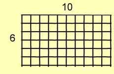
Do you recall from grade school that you find the area of a rectangle by multiplying the lengths of the two sides?

Believe it or not, that's all you need to know to figure out genotype frequencies from allele frequencies.  .

First, let's begin by seeing how multiplying the sides of a rectangle to find its area is just like polynomial multiplication in algebra.

For example, consider a rectangle with sides of 6 and 10.  The area, of course, is: 6 x 10 = 60
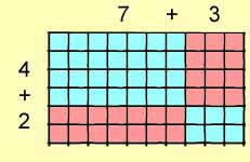
Now consider that each side may be subdivided.  For example, 6 = ( 4 + 2 ) and 10 = (7 + 3 ). 6 x 10 = ( 4 + 2 ) x ( 7 + 3 )            = ( 4 x 7 ) + ( 4 x 3 ) + ( 2 x 7 ) + ( 2 x 3 )            = 28 + 12 + 14 + 6            = 60
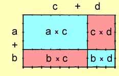
More generally, any rectangle may be composed of four smaller rectangles, each the product of segments along its sides. ( a + b ) x ( c + d ) =         ( a x c ) + ( c x d ) + ( b x c ) + ( b x d )

Now let's apply this geometric multiplication to population genetics.  Just imagine all the individuals comprising a population to be arranged into a square array.  Our tool for doing this is the Punnett Square.

(Here is an irrelevant mathematical aside on the Pythagorean theorem, just for fun.)

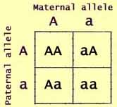
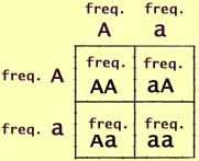
The Punnett Square

The Punnett square was introduced by English geneticist Reginald Crundall Punnett as a tool for visualizing genetic combinations.

In its simplest form, a Punnett square shows how alleles combine to form genotypes.

Along one side of the square are listed the alleles that a zygote may receive from its mother.  Along the other side are listed the alleles that the zygote may receive from its father.  Within each square are listed the resulting genotypes.
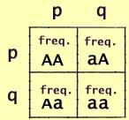
However, instead of just listing alleles and genotypes, the sides of our square can represent the allele frequencies.  Then the boxes represent the genotype frequencies. But now this becomes more than a simple listing.  The square can now be used for computation.
We can now substitute algebraic or numerical representations of allele and genotype frequencies.: p is the frequency of A and q is the frequency of a.
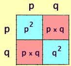
Finally we use multiplication by geometry, just like in the rectangle above, to see that: [freq AA] = p2 [freq Aa] = 2pq   [freq aa] = q2
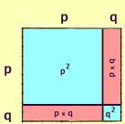
This may appear just a bit more intuitive if we make the segments along the sides of the square proportional to the allele frequency. As shown at right, p = 0.8 and q = 0.2 )

Notes for chapter 1 / 2 / 3 / 4 / 5 / 6 / 7 / 8 / 9 / 10 / 11 / 12 / 13 / 14 / 15 / 16 / 17

The utility of algebra-by-geometry is not limited to Punnett Squares. Here is an elegant proof of the Pythagorean Theorem from Euclidean geometry.  You remember, "In any right triangle, the square of the hypotenuse is equal to the sum of the squares of the other two sides."

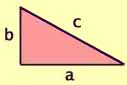
Take any right triangle with sides a and b and hypotenuse c. Area = 1/2 x ab
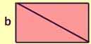
Put two of these triangles together to form a rectangle.  Area = 2 x (1/2 x ab)
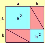
Next, arrange two such rectangles into a larger square with side a + b. Clearly, the area of this larger square is equal to four of the triangles plus the two blue squares. Area = (a + b)2 = a2 + b2 + [4 x (1/2 x ab)]
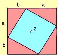
Now rearrange the four pink triangles within the same larger square.  The side of the outer square is still (a + b), so the area of the outer square also still (a + b)2. Area = = c2 + [4 x (1/2 x ab)] Since the larger square has not changed its size (side a + b), and there are still four pink triangles, the blue areas must also remain equal.  Thus the sum of the areas of the two blue squares in the diagram above must equal area of the single blue square in this diagram.   Therefore, a2 + b2 = c2

In words, the square of the hypotenuse ( c² ) is equal to the sum of the squares
(a² + b² ) of the other two sides.

Now, back to evolution...

Notes for chapter 1 / 2 / 3 / 4 / 5 / 6 / 7 / 8 / 9 / 10 / 11 / 12 / 13 / 14 / 15 / 16 / 17

  304 index page

Comments and questions: dgking@siu.edu
Department of Zoology e-mail: zoology@zoology.siu.edu
Comments and questions related to web server: webmaster@science.siu.edu